单细胞免疫组库VDJ| 从零开始scRepertoire分析,解决真实场景中可能的问题
选择既有RNA又有TCR样本的数据进行后续分析。重点解决以下三个小问题
1,只看TCR时(二),不同样本,不同分组情况下的clone差异以及变化;
2,TCR结合转录组数据(三 四),展示clone的分布可视化 以及 不同celltype中clone的差异以及变化;
3,一些可能的报错:(1)结合单细胞数据时;(2)官网链接中一些group相关的函数,按照推文或者使用??查看报错函数的具体说明
一 准备R包,数据集
安装scRepertoire包,如果出现如下的Error,按照提示安装gsl后再安装scRepertoire。
BiocManager::install("scRepertoire")suppressMessages(library(scRepertoire))#Error: package or namespace load failed for 'scRepertoire’ in loadNamespace(i, c(lib.loc, .libPaths()), versionCheck = vI[[i]]):# 不存在叫'gsl’这个名字的程辑包#install.packages("gsl")suppressMessages(library(Seurat))library(ggsci)
二 scRepertoire VDJ分析
1,处理VDJ数据
使用combineTCR函数结合所有样本的filtered_contig_annotations.csv数据,使用samples 和 ID 函数对样本进行标注和分组
S1 <- read.csv("./scTCR_data/t2_Normal.filtered_contig_annotations.csv")S2 <- read.csv("./scTCR_data/t2_PBMC.filtered_contig_annotations.csv")S3 <- read.csv("./scTCR_data/t3_Normal.filtered_contig_annotations.csv")S4 <- read.csv("./scTCR_data/t3_PBMC.filtered_contig_annotations.csv")S5 <- read.csv("./scTCR_data/t3_Center.filtered_contig_annotations.csv")S6 <- read.csv("./scTCR_data/t4_Normal.filtered_contig_annotations.csv")S7 <- read.csv("./scTCR_data/t4_PBMC.filtered_contig_annotations.csv")S8 <- read.csv("./scTCR_data/t4_Center.filtered_contig_annotations.csv")S9 <- read.csv("./scTCR_data/UT1_Normal.filtered_contig_annotations.csv")
contig_list <- list(S1, S2, S3, S4, S5, S6, S7,S8,S9)
combined <- combineTCR(contig_list,
samples = c("t2", "t2", "t3", "t3","t3","t4", "t4", "t4", "UT1"), ID = c("Normal", "PBMC", "Normal", "PBMC","Center", "Normal", "PBMC", "Center","Normal"),
cells ="T-AB")
也可以使用addVariable函数添加其他信息,如tissue ,age ,分期等,这个很实用,后续可以使用这些分组进行 clone 的各类比较
example <- addVariable(combined, name = "Tissue",
variables = c("Tumor", "Tumor", "Tumor", "Tumor","Tumor", "Tumor", "Tumor", "Tumor","Normal"))example[[1]][1:5,]
2,VCJ分析以及可视化
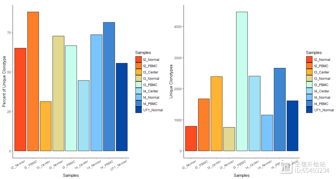
2.1 Quantify Clonotypes 探索克隆型
使用quantContig 探索每个样本的unique clone信息(分别为比例 以及 个数)
p1 <- quantContig(combined, cloneCall="gene nt", scale = T) theme(axis.text.x = element_text(angle = 30,vjust = 0.85,hjust = 0.75))#X坐标加点斜体,出图好看p2 <- quantContig(combined, cloneCall="gene nt", scale = F) theme(axis.text.x = element_text(angle = 30,vjust = 0.85,hjust = 0.75))p1 p2
注:这里cloneCall函数有四个参数
(1) “gene” :使用包含 TCR/Ig 的 VDJC 基因
(2) “nt”:使用 CDR3 区域的核苷酸序列
(3) “aa” :使用 CDR3 区域的氨基酸序列
(4) “gene nt” 使用包含 TCR/Ig CDR3 区域的核苷酸序列的 VDJC 基因
柱形图具体的数值可以添加exportTable = T函数导出
quantContig_output <- quantContig(combined, cloneCall="gene nt",
scale = T, exportTable = T)quantContig_output contigs
values total scaled
1
795 t2_Normal 1221 65.11057
2
1672
t2_PBMC 1903 87.86127
3
759 t3_Normal 1044 72.70115
4
4462
t3_PBMC 6695 66.64675
5
2387 t3_Center 7615 31.34603
6
1159 t4_Normal 1575 73.58730
7
2661
t4_PBMC 3274 81.27673
8
2403 t4_Center 5395 44.54124
9
1618 UT1_Normal 2918 55.44894
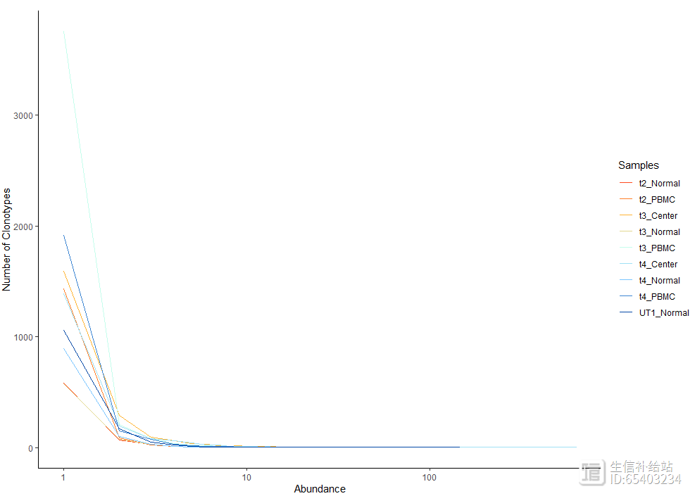
2.2 Clonotype Abundance克隆型丰度
使用abundanceContig函数 查看各个样本的克隆型总数的折线图,也可以添加exportTable = T函数输出折线图的具体结果
abundanceContig(combined, cloneCall = "gene", scale = F)
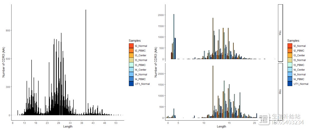
2.3 Length of Clonotypes克隆型长度
使用lengtheContig函数查看 CDR3 序列的长度分布。chain 函数可以选择是如左图的全部展示,还是如右图的TRA ,TRB分别展示
p11 <- lengthContig(combined, cloneCall="aa", chain = "combined")#左图p22 <- lengthContig(combined, cloneCall="aa", chain = "single") #右图p11 p22
2.4 Compare Clonotypes比较克隆型
使用compareClonotypes函数查看样本之间的克隆型的比例和动态变化。cloneCall可以选择“gene nt”
compareClonotypes(combined, numbers = 10,
samples = c("t3_PBMC","t3_Normal","t3_Center"),
#samples = c("t2_Normal", "t2_PBMC","t3_PBMC","t3_Normal","t3_Center"),
cloneCall="aa",
graph = "alluvial")
samples可以选择任意样本,但是如果top number clonotype sequences之间没有共享的话,则没有连线。

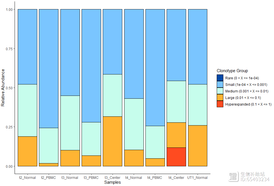
2.5 Clonal Space Homeostasis克隆空间稳态
可以通过clonalHomeostasis函数查看, 各特定比例的克隆型(cloneTypes:Rare,,,Hyperexpanded)所占据该样本的相对比例
clonalHomeostasis(combined, cloneCall = "gene",cloneTypes = c(Rare = 1e-04,Small = 0.001,Medium = 0.01,Large = 0.1,Hyperexpanded = 1))
2.6 Clonal Proportion 克隆比例
可以通过clonalProportion函数查看克隆型的比例,按克隆型的出现频率将其进行排名,1:10表示每个样本中的前10个克隆型。
clonalProportion(combined, cloneCall = "nt")

2.7 Overlap Analysis 重叠分析
使用clonalOverlap函数分析样本之间的相似性,使用 clonesizeDistribution函数对样本进行聚类。
clonalOverlap(combined, cloneCall = "gene nt",
method = "overlap")
clonesizeDistribution(combined,
cloneCall = "gene nt",
method="ward.D2")

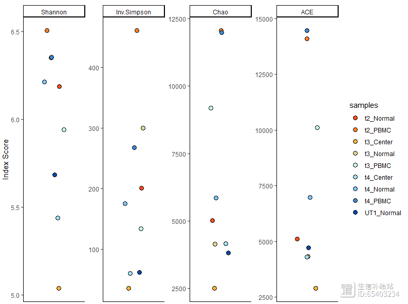
2.8 Diversity Analysis多样性分析
使用clonalDiversity函数进行多样性分析,会通过以下4各指标计算:
1)Shannon, 2) inverse Simpson, 3) Chao1和4)based Coverage Estimator (ACE)。
前两者一般用于估计基线多样性,Chao/ACE 指数用于估计样本的丰富度。
clonalDiversity(combined,
cloneCall = "gene nt",
n.boots = 100)
clonalDiversity(combined,
cloneCall = "gene nt",
group = "ID",
n.boots = 100)
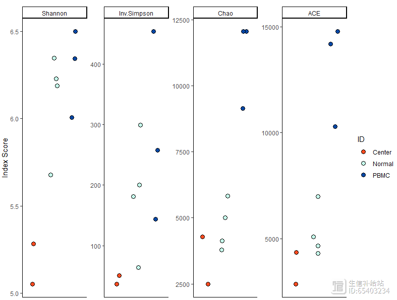
注意此处不要用group.by 而是要用group 。
三 scRepertoire-VDJ RNA
以上即为单细胞免疫组库的常规分析,我们更多的还是与scRNA-seq数据结合,就可以在umap上查看clone的分布情况 以及 基于cluster/celltype展示clonotype的分布情况。
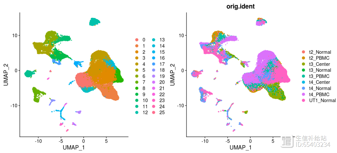
3.1 Seurat标准流程
folders的样本文件夹内为cellranger的3个标准文件,的简单的走一遍标准流程单细胞工具箱|Seurat官网标准流程,此处仅为示例就不考虑批次问题了。
folders=list.files('./')folders#[1] "t2_Normal" "t2_PBMC"
"t3_Center" "t3_Normal" "t3_PBMC"
"t4_Center" "t4_Normal" "t4_PBMC"
"UT1_Normal"
#批量读取10X单细胞转录组数据文件夹sceList = lapply(folders,function(folder){ CreateSeuratObject(counts = Read10X(folder),
project = folder )})sce.all <- merge(sceList[[1]],
y = c(sceList[[2]],sceList[[3]],sceList[[4]],
sceList[[5]],sceList[[6]],sceList[[7]],sceList[[8]],sceList[[9]]),
add.cell.ids = folders, #添加样本名
project = "scRNA")sce.all #查看#线粒体比例sce.all[["percent.mt"]] <- PercentageFeatureSet(sce.all, pattern = "^MT-")#过滤sce <- subset(sce.all, subset = nFeature_RNA > 500 &
nFeature_RNA < 5000 &
percent.mt < 20)VlnPlot(sce, features = c("nFeature_RNA", "nCount_RNA", "percent.mt"), ncol = 3)#标准化sce <- NormalizeData(sce)#高变基因sce <- FindVariableFeatures(sce, selection.method = "vst", nfeatures = 2000)all.genes <- rownames(sce)#归一化sce <- ScaleData(sce, features = all.genes)#降维聚类sce <- RunPCA(sce, npcs = 50)sce <- FindNeighbors(sce, dims = 1:30)sce <- FindClusters(sce, resolution = 0.5)sce <- RunUMAP(sce, dims = 1:30)sce <- RunTSNE(sce, dims = 1:30)p1 <- DimPlot(sce, reduction = "umap", pt.size=0.5, label = F,repel = TRUE)p2 <- DimPlot(sce, reduction = "umap",group.by = "orig.ident", pt.size=0.5, label = F,repel = TRUE)p1 p2
(1) 添加meta,处理barcode
读取文章提供的meta信息,如下图所示,红框中的不一致的部分需要tidyverse处理一下Tidyverse|数据列的分分合合,一分多,多合一
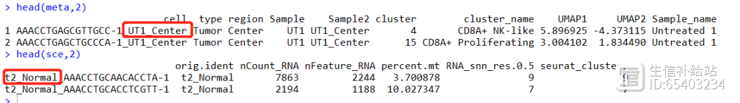
meta <- read.table("ccRCC_6pat_cell_annotations.txt",
sep = "\t",header = T)meta2 <- meta %>% separate(cell,into = c( "CB","sample","pos"),sep = "_") %>% mutate(cell = paste(sample,pos,CB,sep = "_"))
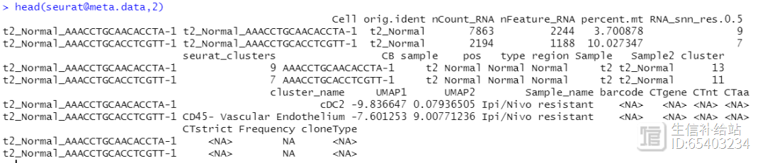
sce@meta.data <- sce@meta.data %>% rownames_to_column("cell") %>% inner_join(meta2,by = "cell") %>% column_to_rownames("cell")head(sce@meta.data)#
orig.ident nCount_RNA nFeature_RNA percent.mt RNA_snn_res.0.5 seurat_clusters
CB#t2_Normal_AAACCTGCAACACCTA-1 t2_Normal
7863
2244 3.700878
9
9 AAACCTGCAACACCTA-1#t2_Normal_AAACCTGCACCTCGTT-1 t2_Normal
2194
1188 10.027347
7
7 AAACCTGCACCTCGTT-1#
sample
pos type region Sample Sample2 cluster
cluster_name
UMAP1
UMAP2#t2_Normal_AAACCTGCAACACCTA-1
t2 Normal Normal Normal
t2 t2_Normal
13
cDC2 -9.836647 0.07936505#t2_Normal_AAACCTGCACCTCGTT-1
t2 Normal Normal Normal
t2 t2_Normal
11 CD45- Vascular Endothelium -7.601253 9.00771236#
Sample_name#t2_Normal_AAACCTGCAACACCTA-1 Ipi/Nivo resistant#t2_Normal_AAACCTGCACCTCGTT-1 Ipi/Nivo resistant
(2) sce的细胞数 和 meta信息 不一致
因为前面Seurat流程使用的自己的参数,而meta信息是文章给的。

解决:使用subset函数 提取 meta.data中的cell
sce@meta.data <- sce@meta.data %>% rownames_to_column("Cell") %>% mutate(Cell2 = Cell) %>% column_to_rownames("Cell2")sce <- subset(sce,Cell %in% sce@meta.data$Cell)
3.2 VDJ结果结合RNA
使用combineExpression函数将VDJ结果和 RNA结果结合。
注:combined的barcode 和 sce的rownames 一定要一致,有出入的使用tidyverse包进行数据处理。
seurat <- combineExpression(combined, sce,
cloneCall="gene",
# group.by = "Sample",
proportion = FALSE,
cloneTypes=c(Single=1, Small=5, Medium=20, Large=100, Hyperexpanded=500))head(seurat)
因为很多barcode 并没有TCR clone ,因此cloneTypes 含有一些NA是正常的 。
3.3 clonoType umap分布
可以使用DimPlot函数 绘制 clonetype在UUMAP中的分布
colorblind_vector <- colorRampPalette(rev(c("#0D0887FF", "#47039FFF",
"#7301A8FF", "#9C179EFF", "#BD3786FF", "#D8576BFF",
"#ED7953FF","#FA9E3BFF", "#FDC926FF", "#F0F921FF")))p111 <- DimPlot(seurat, group.by = "cluster_name",label = T)p222 <- DimPlot(seurat, group.by = "cloneType",label = T) #NoLegend() scale_color_manual(values=colorblind_vector(5)) theme(plot.title = element_blank())p111 p222
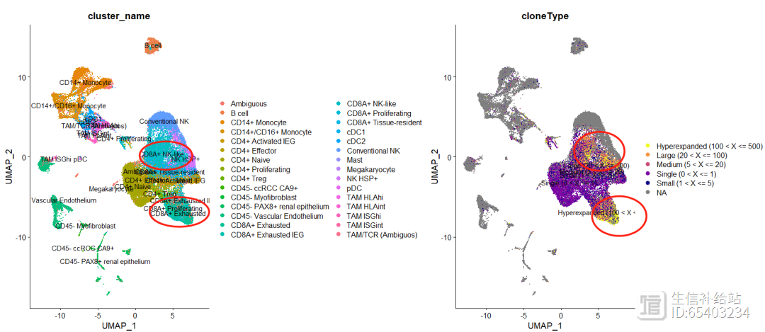
可以大概看出来CD8细胞中clone更多,符合文献的研究结果。
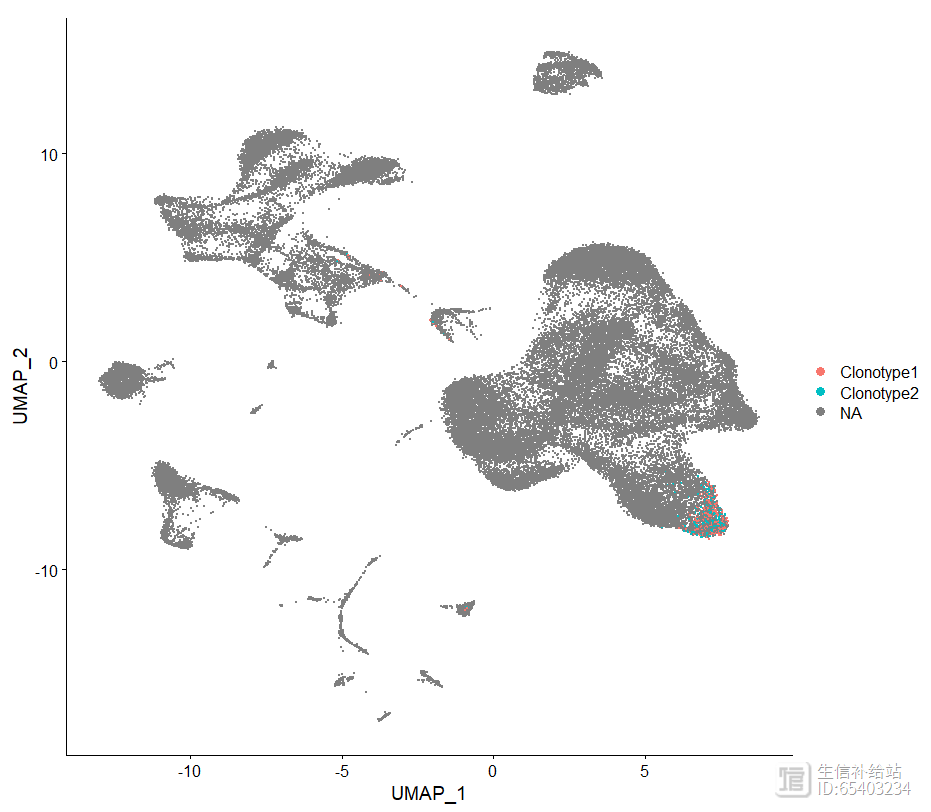
3.4 highlightClonotypes 高亮特定克隆型
使用highlightClonotypes函数 展示特定序列的克隆型分布
seurat <- highlightClonotypes(seurat,
cloneCall= "aa",
sequence = c("CAVGGRSNSGYALNF;CAASRNNNDMRF_CASSSLGNEQFF",
"CAASRNNNDMRF_CASSSLGNEQFF"))DimPlot(seurat, group.by = "highlight") theme(plot.title = element_blank())
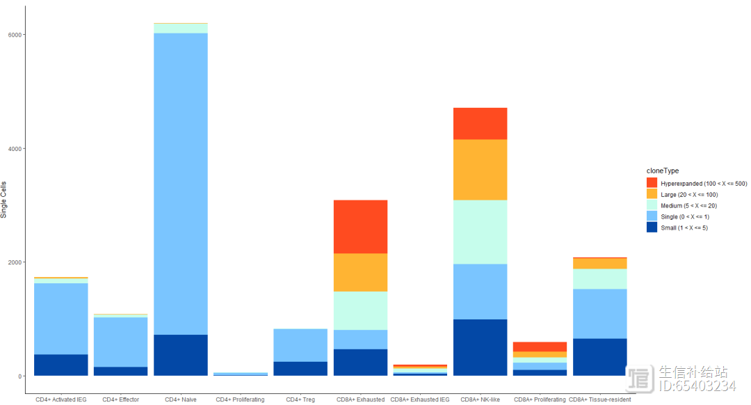
3.5 occupiedscRepertoire cloneType分布
查看CD8T和 CD4T细胞中cloneType的分布情况
seurat_T <- subset(seurat, cluster_name %in% c("CD8A Exhausted","CD8A Exhausted IEG",
"CD8A NK-like","CD8A Proliferating","CD8A Tissue-resident",
"CD4 Activated IEG","CD4 Effector" ,"CD4 Naive","CD4 Proliferating" ,
"CD4 Treg") )
occupiedscRepertoire(seurat_T, x.axis = "cluster_name")
3.6 alluvialClonotypes
使用alluvialClonotypes函数绘制T细胞种各个celltype之间的clonetype信息的桑葚图
alluvialClonotypes(seurat_T, cloneCall = "gene",
y.axes = c("cluster_name", "cloneType"),
color = "cluster_name")

3.7 getCirclize
使用getCirclize函数绘制circos图
library(circlize)library(scales)circles <- getCirclize(seurat,
cloneCall = "gene nt",
groupBy = "cluster_name"
)

四 scRepertoire基于celltype
第二部分中是根据sample计算的clone的一系列指标,如克隆型分布,长度,空间稳态等 。那经过第三部分中和单细胞转录组结合后就可以根据celltype维度进行clone的上述所有统计,这里仅示例几个。
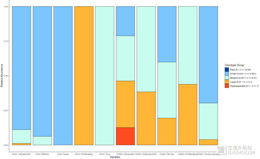
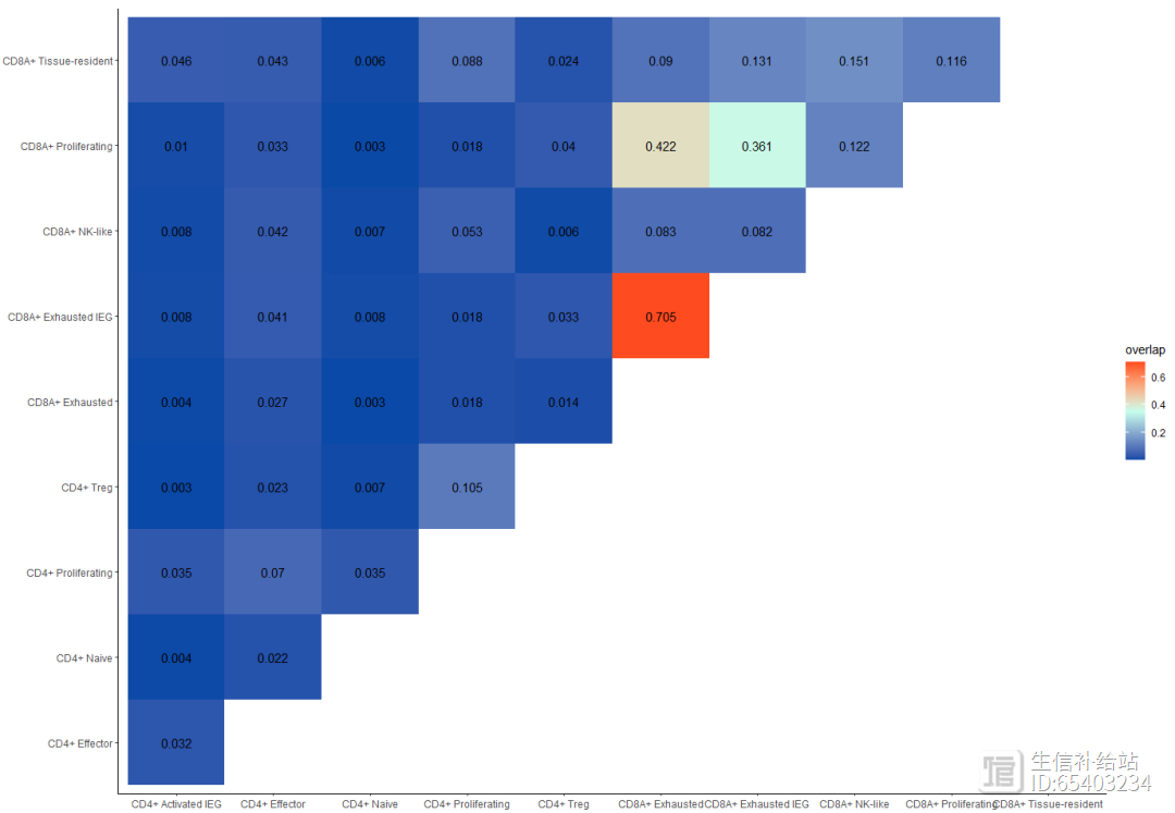
4.1 按照celltype拆分
首先使用expression2List函数将seurat按照cluster_name进行拆分,然后就可进行二中的所有分析 。
注意这里不是官网的split.by ,而要使用group
combined2 <- expression2List(seurat_T,
group = "cluster_name")length(combined2) p01 <- clonalDiversity(combined2,
cloneCall = "nt")p02 <- clonalHomeostasis(combined2,
cloneCall = "nt")p03 <- clonalOverlap(combined2,
cloneCall="aa",
method="overlap")p01p02#保存数据(后台获取),以备后用save(combined,seurat_T,file = "combined_seurat_T.RData")
官网:/vignettes/vignette.html
- 0000
- 0000


 0000
0000

 0000
0000- 0002